Euler Examples

Search

The Riemann Sphere

The Riemann Sphere is a representation of the compactified (with infinity) complex plane on the sphere with center (0,0,1/2) and radius 1/2.

It uses the so-called stereographic projection from the north pole (0,0,1) through the sphere to the x-y-plane of points (x,y,0). A little geometry reveals the following equation

>function px(x,y,z) &= x/(1-z)

                                  x
                                -----
                                1 - z

>function py(x,y,z) &= y/(1-z)

                                  y
                                -----
                                1 - z

To compute the inverse function, we use the "solve" function of Maxima. Thus we solve

under condition that (x,y,z) is on the sphere. There are two solutions. One of them is the north pole (0,0,1) and discard this solution.

>xyz &= solve([x^2+y^2+(z-1/2)^2=1/4,tx=px(x,y,z),ty=py(x,y,z)],[x,y,z])[2]

                                                      2     2
                 tx                 ty              ty  + tx
       [x = -------------, y = -------------, z = -------------]
              2     2            2     2            2     2
            ty  + tx  + 1      ty  + tx  + 1      ty  + tx  + 1

Now we define the components of the inverse function.

>function qx(tx,ty) &= x with xyz

                                 tx
                            -------------
                              2     2
                            ty  + tx  + 1

>function qy(tx,ty) &= y with xyz

                                 ty
                            -------------
                              2     2
                            ty  + tx  + 1

>function qz(tx,ty) &= z with xyz

                                2     2
                              ty  + tx
                            -------------
                              2     2
                            ty  + tx  + 1

We now want to draw a grid on the sphere with the usual longitudinal and equilateral circles. We use a very dense grid to get a smooth representation.

If the grid is projected to the plane the result will be a grid with radials and circles. The radii of the circles are computed using the projection "px" from above.

>t=linspace(0,2pi,240)';
>s=(1:119)*pi/120; r=px(sin(s),0,cos(s));
>w=r*exp(I*t);
>plot2d(w,r=11,cgrid=10):

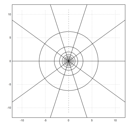
This is the projection of the grid on the ball to the plane. Note "cgrid" which is a way to reduce the grid lines that are actually drawn for a complex grid matrix.

To draw the grid on the ball, we use the inverse projection.

>tx=re(w); ty=im(w);
>x=qx(tx,ty); y=qy(tx,ty); z=qz(tx,ty);
>plot3d(x,y,z,grid=[20,10],>hue):

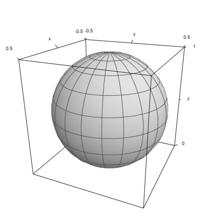
Note that the surface has a very fine resolution, but we draw only 20 and 10 grid lines in each direction.

Let us now distort the grid with a Möbius transformation. We plot the distorted grid back on the sphere.

>wm=(w+1)/(w+2);
>tx=re(wm); ty=im(wm);
>x=qx(tx,ty); y=qy(tx,ty); z=qz(tx,ty);
>plot3d(x,y,z,grid=[20,10],>hue,angle=100°,height=10°,<frame,zoom=4.5):

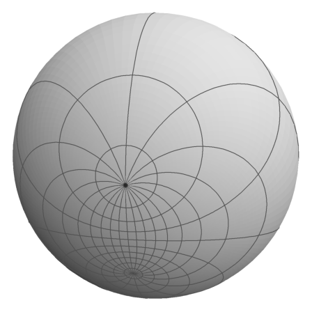
The Möbius transformation maps infinity to 1 and 0 to 1/2. Projecting back we get the two points on the sphere in the image above.

The Stereographic Projection and Povray

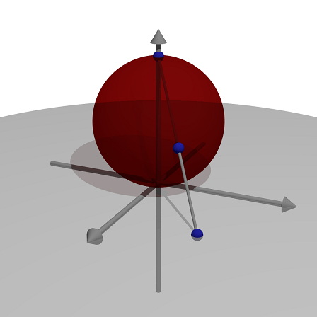
We can use Povray to visualize the stereographic projection. For this, Povray must be installed completely, and the path to "pvengine.exe" must be in the system path, or the variable "defaultpovray" must be set in EMT.

>load povray

Functions to generate Povray files for the open Raytracer. 

We start the Povray scene and set the zoom and the center point.

>povstart(zoom=4.8,center=[0,0,0.2]);

The first element is a red, half transparent sphere.

>writeln(povsphere([0,0,1/2],1/2,povlook(red,transparent=0.8)));

The next element is a transparent, gray plane which represents the x-y-plane. It is bounded by cylinder with radius 2.4.

>box=povcylinder([0,0,-2],[0,0,2],2.4,look="");
>writeln(povplane([0,0,1],0,povlook(lightgray,transparent=0.5),box));

The next elements are three blue points.

>writeln(povpoint([0,0,1],povlook(blue),0.04));
>x=0.7; y=0.6; 
>writeln(povpoint([x,y,0],povlook(blue),0.04));
>r=x^2+y^2+1; xp=x/r; yp=y/r; zp=(x^2+y^2)/r;
>writeln(povpoint([xp,yp,zp],povlook(blue),0.04));

Then there is a segment in gray, connecting the North pole to the point in the x-y-plane.

>writeln(povsegment([x,y,0],[0,0,1],povlook(gray),0.01));

Then we want the coordinate axes.

>writeln(povarrow([-1,0,0],[2,0,0],povlook(gray)));
>writeln(povarrow([0,-1,0],[0,2,0],povlook(gray)));
>writeln(povarrow([0,0,-1],[0,0,2.1],povlook(gray)));

THe following ends the scene and generates an image with a high resolution.

>povend(h=1000,w=1000);

Examples